Chapter 4 Decision Tree
4.1 Model Visualization
## [1] 0.7756755The plot visualized our regression tree model. Since the size of the tree is so large, visualization does not work here. But we can find out each node’s information and splitting rule by checking the summary of tree model.
4.2 Model Evaluation
##       MSE      MAE R-Squared
## 1 1567.24 19.46132 0.5838036
The evaluation table shows regression tree’s performance on the test set, comparing with linear model, tree model has much better performance no matter which criterion we use. Hence, in terms of accuracy, decision tree would be my choice.
4.3 Model Interpretation
4.3.1 Partial Dependence Plot
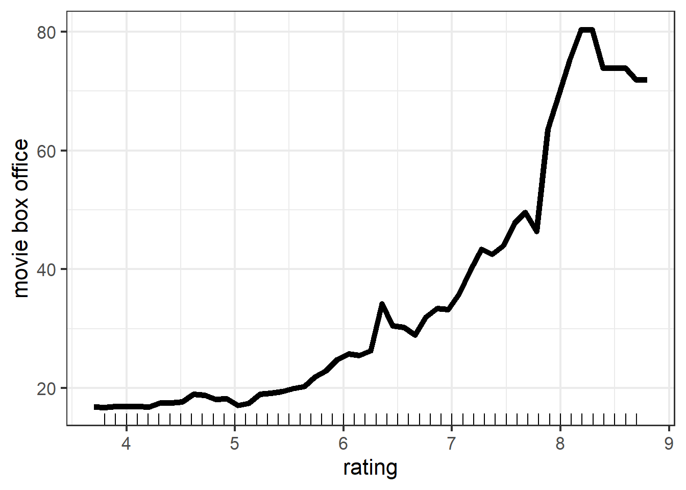
Comparing the PDP of rating by using tree model and linear model, we find that the overall trend is the same, i.e., as rating goes up, predicted movie box office rises. And one difference is that, instead of being a straight line in linear model, we can observe that the line in tree model has ups and downs. This is because in tree model, the relationship between rating and gross does not have to be linear. Clearly, the latter is what we observed in reality. More insights that we can derive from this plot is that as rating increases from 4 to 6, movie box office does not increase a lot. This is probably because for those movies, people would watch and rate them online, but are not willing to buy tickets to watch them in theater. Hence, they all tend to have few box office. As for why there is a huge jump when rating increased from 7.9 to 8.3, I find it hard to give a reasonable guess.
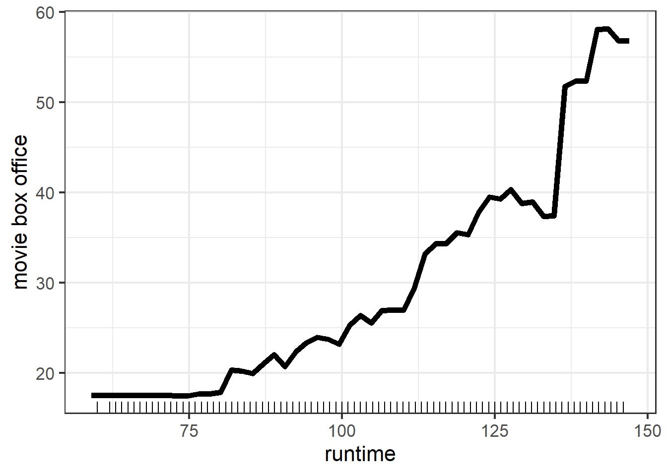
Again, the consistence and difference between PDP of runtime by using tree model and linear model is similar to what we get at rating part: the overall trend is the same and we can get more insights from tree model. One more thing to notice is that, the range of movie box office in tree model for the two different features are not as much as it in linear model. This suggests that rating and runtime in tree model may contribute relatively equal explanations for variations in response variable.
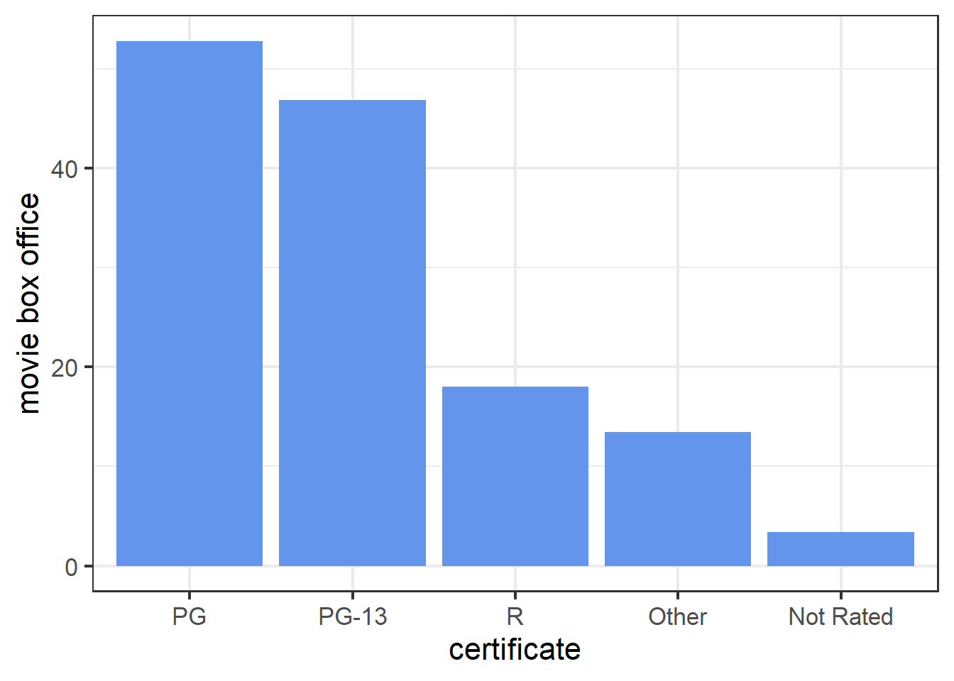
The PDP of certificate in tree model shows that PG and PG-13 movies tend to have more box office while Not Rated movies tend to have less box office. This is similar to the results obtained from linear model.
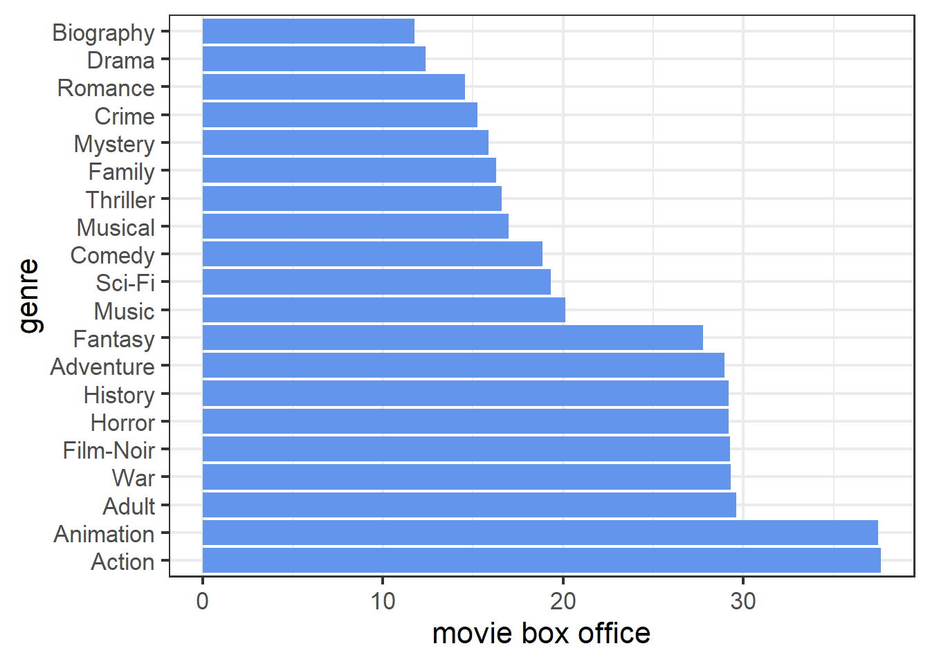
The PDP of genre in tree model shows that action, animation, and horror movies are top three most popular types while drama, biography, and romance are the three types with least audience. In general, this is consistent with the conclusion by using linear model. But note that, the difference between each genre in tree model are far less than the difference in linear model. This indicates that genre in tree model is not as much important as it is in linear model (later by drawing the feature importance plot, we find the genre is least important in tree model while it is the second important in linear model).
4.3.2 Local Interpretable Model-agnostic Explanations (LIME)
| model_intercept | model_prediction | feature | feature_value | feature_weight | feature_desc | prediction |
|---|---|---|---|---|---|---|
| -24.77 | 111.018 | year | 27 | 24.136 | year = 1996 | 8.625 |
| -24.77 | 111.018 | certificate | 3 | 52.221 | certificate = PG | 8.625 |
| -24.77 | 111.018 | runtime | 100 | 46.472 | runtime <= 232 | 8.625 |
| -24.77 | 111.018 | genre | 1 | 36.028 | genre = Action | 8.625 |
| -24.77 | 111.018 | rating | 5 | -23.069 | 3.27 < rating <= 5.25 | 8.625 |
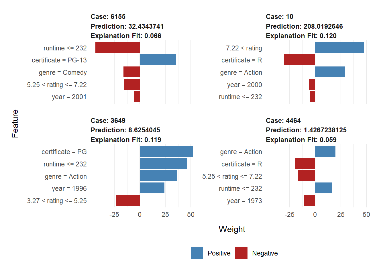
From the explanation table, we have that the local model for case 3649 is \(\hat{y}_{lime} = -22.479 -24.341 \cdot \mathbf{1}_{3.27 < rating <= 5.25}+61.044 \cdot \mathbf{1}_{certificate = PG}+33.229 \cdot \mathbf{1}_{genre = Action}+44.626 \cdot \mathbf{1}_{runtime <= 232}+41.078 \cdot \mathbf{1}_{year = 1996}\). By comparing this result with lime model get in linear part, we find that even the direction of the effect of some features changed. For example, \(runtime\leq232\) has a negative contribution to prediction in linear part, but it has a positive contribution here. Another difference is that the feature weight also changed a lot, certificate in linear part only rank as the third one but has the largest weight here. Since in linear part, the interpretation given by local model and ordinary linear model are in general consistent, my guess about the difference between two local models is that they are just the representation of the original models, i.e., the linear model and the tree model gives different prediction for the same data points, and this is reflected on difference of local models.
##   lime error original error
## 1  -33.19643     -13.082431
## 2  106.24943     -20.313573
## 3  -96.67111       8.675889
## 4  -33.11856       1.751440
The residual table shows that our tree model also outperforms its local model. Also note that the error for each case in tree model is also less than it in linear model.
4.3.2.1 Gower Distance
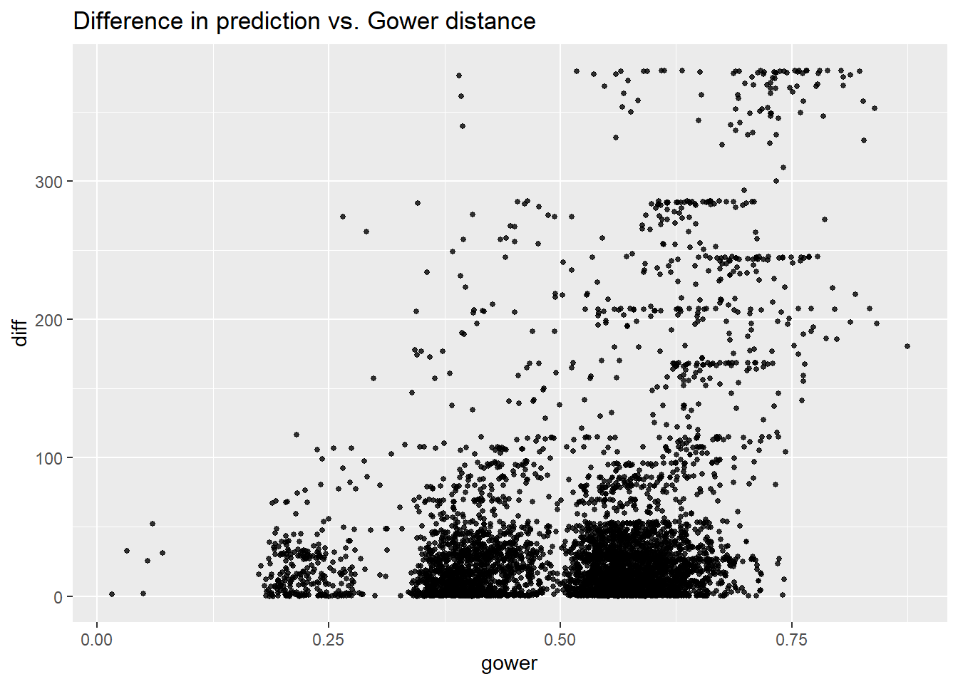
From the plot, we still have that as Gower distance increases, the variance of difference between pairs increases. One major distinction from linear part is that for pairs at the same difference level (the Gower distance is same), tree model tend to make more variant predictions compared with linear model. In my opinion, I think this might be an advantage since considering the features we include, two movies defined as similar will just have common characteristics in terms of rate, run time, genre, certificate, and released year. But for movies with even all the same features mentioned above, in real case, they still tend to have very different box office as many other factors could have impact on, such as season, published area, and published volume in cinema every day.
4.3.3 Shapley Additive Explanations
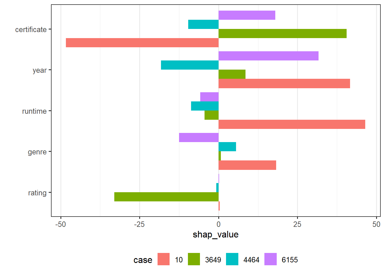
From the SHAP plot, case 10 has the most prediction value, runtime and rating contribute majority of the difference between mean gross and prediction of case 10. By checking the feature value of each case in our sample, we find that case 10 has the highest rate and longest run time. On the other hand, case 4464 has the least prediction value, year is the main factor caused the low prediction. And we can see that case 4464 is the oldest movie which is published in 1973. By comparing the interpretation provided by SHAP and by LIME, they seems to be not consistent with each other for some features. For example, for case 10, LIME implies that runtime has a negative effect on predicted value while SHAP indicates that runtime has a positive effect. In this particular case, it seems that SHAP’s explanation is more plausible since although case 10 has a run time less than 232 minutes, we can check that its run time is 155 minutes which is larger than most movies in our data set. Hence, runtime should make positive contribution for case 10. The question is, in general, SHAP and LIME, which one provides a more reasonable interpretation or does it depend on situation and purpose.
4.3.4 Feature Importance
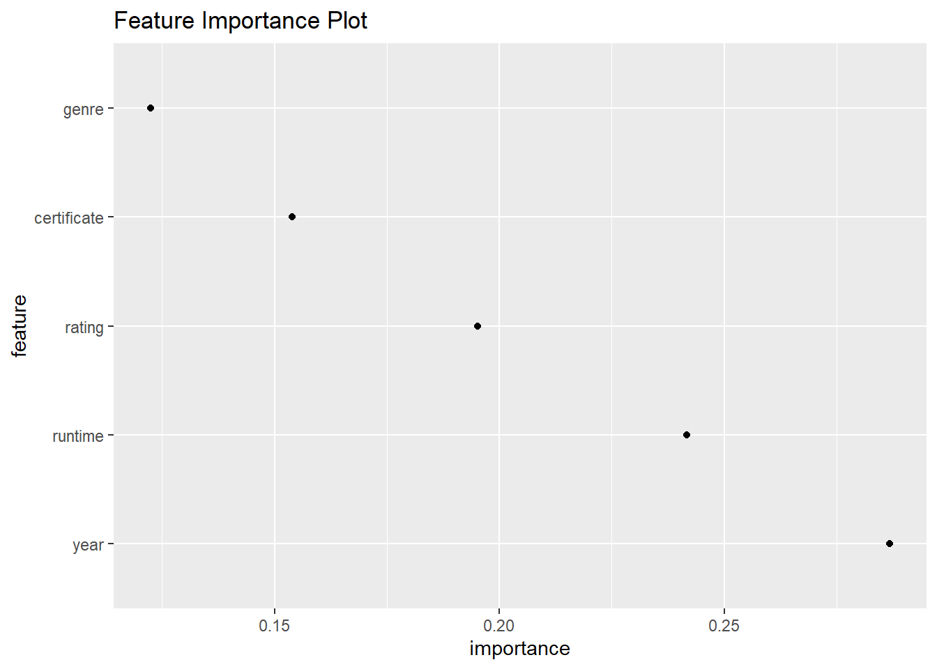
The feature importance plot shows that year is the most important feature while genre is the least important feature. This seems to be consistent with result obtained from partial dependence plot. When compared with feature importance in linear model, they are quiet different. Year in linear model is not as important as it is in tree model. My opinion is that the relationship between year and gross is not linear but will fluctuate, hence linear model could not capture the impact of year. But linear constraint is not a problem for tree model, hence tree model could utilize this feature well.